9 Matrices

In R, a matrix is a vector, with two additional attributes: The number of rows, and the number of columns

As with vectors, every element of a matrix must be of the same mode ; either purely numeric, or purely text, etc.

Creating a matrix from a vector

Given a vector, convert it to a matrix by specifying the number of rows and columns.

m <- matrix( c(1,2,3,4), nrow=2, ncol=2)
m

     [,1] [,2]
[1,]    1    3
[2,]    2    4

Properties

attributes(m)

$dim
[1] 2 2

dim(m)

[1] 2 2

class(m)

[1] "matrix" "array"

Column-major and row-major ordering

Note that by default, the columns of the matrix are filled with the vector’s elements, in the so-called column-major order.

matrix(1:6, nrow=3, ncol=2)

     [,1] [,2]
[1,]    1    4
[2,]    2    5
[3,]    3    6

To force a row-major order instead, set the byrow parameter to TRUE.

matrix( 1:6, nrow=3, ncol=2, byrow=TRUE )

     [,1] [,2]
[1,]    1    2
[2,]    3    4
[3,]    5    6

If we provide only nrow or only ncol, the unspecified parameter will be determined using the length of the vector.

matrix( 1:6, nrow=2 )

     [,1] [,2] [,3]
[1,]    1    3    5
[2,]    2    4    6

matrix( 1:6, ncol=3 )

     [,1] [,2] [,3]
[1,]    1    3    5
[2,]    2    4    6

Element recycling

If the specified matrix sizes are not compatible with the vector’s length, the vector is recycled until it fills the matrix.

matrix( 1:5, nrow=2, ncol=4)

Warning in matrix(1:5, nrow = 2, ncol = 4): data length [5] is not a
sub-multiple or multiple of the number of rows [2]

     [,1] [,2] [,3] [,4]
[1,]    1    3    5    2
[2,]    2    4    1    3

The same recycling is done also when one of the shape parameters is omitted.

matrix( 1:5, nrow=2 )

Warning in matrix(1:5, nrow = 2): data length [5] is not a sub-multiple or
multiple of the number of rows [2]

     [,1] [,2] [,3]
[1,]    1    3    5
[2,]    2    4    1

Accessing individual matrix elements

The element in the r-th row and the c-th column of a matrix m can be accessed with the m[r,c] notation.

m <- matrix(1:6, nrow=2)
m

     [,1] [,2] [,3]
[1,]    1    3    5
[2,]    2    4    6

m[1,1]

[1] 1

m[2,3]

[1] 6

Accessing rows and columns

To get the entire r-th row as a vector, we use the m[r,] notation. Similarly, m[,c] gives the column c.

m <- matrix(1:6, nrow=2)
m

     [,1] [,2] [,3]
[1,]    1    3    5
[2,]    2    4    6

m[1,] # first row, all columns

[1] 1 3 5

m[,1]  # first column, all rows

[1] 1 2

Accessing ranges of rows/columns

As with vectors, we can provide a vector of indices to extract a subset of rows or columns.

m <- matrix( 1:12, nrow=3 )
m

     [,1] [,2] [,3] [,4]
[1,]    1    4    7   10
[2,]    2    5    8   11
[3,]    3    6    9   12

Select rows 1 and 2, all columns:

m[1:2,]

     [,1] [,2] [,3] [,4]
[1,]    1    4    7   10
[2,]    2    5    8   11

Select rows 1 and 2, second column only.

m[1:2, 2]

[1] 4 5

Select rows 1 and 2, and columns 1,4 and 3, in that order.

m[1:2, c(1,4,3)]

     [,1] [,2] [,3]
[1,]    1   10    7
[2,]    2   11    8

Excluding some rows and columns

As with vectors, negative indices can be used to get a new matrix with some rows/columns removed.

m <- matrix( 1:12, nrow=3 )
m

     [,1] [,2] [,3] [,4]
[1,]    1    4    7   10
[2,]    2    5    8   11
[3,]    3    6    9   12

Remove 3rd row.

m[-3,]

     [,1] [,2] [,3] [,4]
[1,]    1    4    7   10
[2,]    2    5    8   11

Remove 2nd column

m[,-2]

     [,1] [,2] [,3]
[1,]    1    7   10
[2,]    2    8   11
[3,]    3    9   12

Remove 1st row and 3rd column

m[-1,-3]

     [,1] [,2] [,3]
[1,]    2    5   11
[2,]    3    6   12

Remove columns from 1 to 2.

m[,-1:-2]

     [,1] [,2]
[1,]    7   10
[2,]    8   11
[3,]    9   12

Setting and getting row and column names

The functions rownames() and colnames() are used to set the names for rows and columns, respectively.

m <- matrix( 1:6, nrow=2)
m

     [,1] [,2] [,3]
[1,]    1    3    5
[2,]    2    4    6

rownames(m) <- c("row I", "row II")
colnames(m) <- c("col a", "col b", "col c")
m

       col a col b col c
row I      1     3     5
row II     2     4     6

When called without an assignment, they return the existing names.

rownames(m)

[1] "row I"  "row II"

colnames(m)

[1] "col a" "col b" "col c"

These names provide an alternative method to access matrix elements.

m["row I", "col b"]

[1] 3

m["row I",]

col a col b col c 
    1     3     5

m[,"col a"]

 row I row II 
     1      2

Create a matrix by setting individual elements

Sometimes we may not have all the data at hand at once. It is possible to start with an empty matrix, and fill it up element-by-element.

m <- matrix(nrow=2, ncol=2)
m

     [,1] [,2]
[1,]   NA   NA
[2,]   NA   NA

m[1,1] <- 1
m[2,1] <- 2
m[1,2] <- 3
m[2,2] <- 4
m

     [,1] [,2]
[1,]    1    3
[2,]    2    4

Create a matrix by combining columns or rows

When we have several different vectors, we can combine them in columns using cbind(), or by rows using rbind().

cbind( c(1,2), c(3,4) )

     [,1] [,2]
[1,]    1    3
[2,]    2    4

rbind( c(1,2), c(3,4), c(-2, 6))

     [,1] [,2]
[1,]    1    2
[2,]    3    4
[3,]   -2    6

Add a row or a column to an existing matrix

The functions cbind() and rbind() can also be used to extend an existing matrix.

m <- matrix( 1:4, nrow = 2)
m

     [,1] [,2]
[1,]    1    3
[2,]    2    4

Add a new column at the end of the matrix.

cbind(m, c(10,11))

     [,1] [,2] [,3]
[1,]    1    3   10
[2,]    2    4   11

Add a new column at the beginning of the matrix.

cbind(c(10,11), m)

     [,1] [,2] [,3]
[1,]   10    1    3
[2,]   11    2    4

Add a new row at the end of the matrix

rbind(m, c(10,11))

     [,1] [,2]
[1,]    1    3
[2,]    2    4
[3,]   10   11

Add a new row at the beginning of the matrix.

rbind(c(10,11), m)

     [,1] [,2]
[1,]   10   11
[2,]    1    3
[3,]    2    4

Insert a row or a column into a matrix

Another application of cbind() and rbind() is inserting columns and rows to existing matrices. As with vectors, such insertion is not done on the original matrix. We generate a new matrix using existing rows/columns, combine them with rbind()/cbind(), and reassign to the variable.

m <- matrix( 1:9, nrow=3, ncol=3)
m

     [,1] [,2] [,3]
[1,]    1    4    7
[2,]    2    5    8
[3,]    3    6    9

Insert a row between second and third rows.

rbind(m[1:2,], c(-1, -2, -3), m[3,])

     [,1] [,2] [,3]
[1,]    1    4    7
[2,]    2    5    8
[3,]   -1   -2   -3
[4,]    3    6    9

Insert a column between first and second columns

cbind( m[,1], c(-4,-5,-6), m[,2:3] )

     [,1] [,2] [,3] [,4]
[1,]    1   -4    4    7
[2,]    2   -5    5    8
[3,]    3   -6    6    9

Assign new values to submatrices

A matrix can be changed in-place by selecting a submatrix using index notation, and assigning a new matrix to it.

m <- matrix( 1:9, nrow=3 )
m

     [,1] [,2] [,3]
[1,]    1    4    7
[2,]    2    5    8
[3,]    3    6    9

m[1,1] <- m[1,1] + 1
m

     [,1] [,2] [,3]
[1,]    2    4    7
[2,]    2    5    8
[3,]    3    6    9

m[1,1] <- m[1,1]*m[2,1]
m

     [,1] [,2] [,3]
[1,]    4    4    7
[2,]    2    5    8
[3,]    3    6    9

m[ c(1,2), c(2,3) ] <- matrix(c(20,21,22,23),nrow=2,byrow = T)
m

     [,1] [,2] [,3]
[1,]    4   20   21
[2,]    2   22   23
[3,]    3    6    9

Removing rows and columns

To remove some selected rows or colums, we just use the index notation to specify the rows and columns we want to keep, and assign the result to the variable’s name.

m <- matrix( 1:9, nrow=3 )
m

     [,1] [,2] [,3]
[1,]    1    4    7
[2,]    2    5    8
[3,]    3    6    9

m <- m[c(1,3),c(2,3)] # remove row 2, col 1
m

     [,1] [,2]
[1,]    4    7
[2,]    6    9

m <- matrix( 1:9, nrow=3 )
m <- m[-2,-1] # remove row 2, col 1
m

     [,1] [,2]
[1,]    4    7
[2,]    6    9

Remove 2nd row.

m <- matrix( 1:9, nrow=3 )
m <- m[-2,]
m

     [,1] [,2] [,3]
[1,]    1    4    7
[2,]    3    6    9

Remove 1st column.

m <- matrix( 1:9, nrow=3 )
m <- m[, -1]
m

     [,1] [,2]
[1,]    4    7
[2,]    5    8
[3,]    6    9

Filtering on matrices

m <- matrix( c(2,9,4,7,5,3,6,1,8) , nrow=3 )
m

     [,1] [,2] [,3]
[1,]    2    7    6
[2,]    9    5    1
[3,]    4    3    8

m >= 5

      [,1]  [,2]  [,3]
[1,] FALSE  TRUE  TRUE
[2,]  TRUE  TRUE FALSE
[3,] FALSE FALSE  TRUE

m[m>=5]

[1] 9 7 5 6 8

m[ m<5 ] <- 0
m

     [,1] [,2] [,3]
[1,]    0    7    6
[2,]    9    5    0
[3,]    0    0    8

Matrix operations

Transpose

m <- matrix(1:4, nrow=2)
m

     [,1] [,2]
[1,]    1    3
[2,]    2    4

t(m)

     [,1] [,2]
[1,]    1    2
[2,]    3    4

Elementwise product

     [,1] [,2]
[1,]    1    3
[2,]    2    4

m * m

     [,1] [,2]
[1,]    1    9
[2,]    4   16

Matrix multiplication

     [,1] [,2]
[1,]    1    3
[2,]    2    4

m %*% m

     [,1] [,2]
[1,]    7   15
[2,]   10   22

Multiply by a scalar

     [,1] [,2]
[1,]    1    3
[2,]    2    4

3 * m

     [,1] [,2]
[1,]    3    9
[2,]    6   12

Matrix addition

     [,1] [,2]
[1,]    1    3
[2,]    2    4

m + m

     [,1] [,2]
[1,]    2    6
[2,]    4    8

Sums of rows and columns

m <- matrix( 1:12, nrow=3 )
m

     [,1] [,2] [,3] [,4]
[1,]    1    4    7   10
[2,]    2    5    8   11
[3,]    3    6    9   12

rowSums(m)

[1] 22 26 30

colSums(m)

[1]  6 15 24 33

Averages of rows and columns

     [,1] [,2] [,3] [,4]
[1,]    1    4    7   10
[2,]    2    5    8   11
[3,]    3    6    9   12

rowMeans(m)

[1] 5.5 6.5 7.5

colMeans(m)

[1]  2  5  8 11

Mathematical functions applied on matrices

m <- matrix(1:4, nrow=2)
sqrt(m)

         [,1]     [,2]
[1,] 1.000000 1.732051
[2,] 1.414214 2.000000

sin(m)

          [,1]       [,2]
[1,] 0.8414710  0.1411200
[2,] 0.9092974 -0.7568025

exp(m)

         [,1]     [,2]
[1,] 2.718282 20.08554
[2,] 7.389056 54.59815

log(m)

          [,1]     [,2]
[1,] 0.0000000 1.098612
[2,] 0.6931472 1.386294

The `apply()` function

Suppose you have a function that takes a vector and returns a number.
You want to apply this function to each row (or column) of a matrix.

m <- matrix( 1:9, nrow=3)
m

     [,1] [,2] [,3]
[1,]    1    4    7
[2,]    2    5    8
[3,]    3    6    9

apply(m, 1, mean) # same as rowMeans()

[1] 4 5 6

apply(m, 2, mean) # same as colMeans()

[1] 2 5 8

apply(m,1,prod)

[1]  28  80 162

We can also use apply() with user-defined functions.

inverse_sum <- function(x) sum(1/x)
inverse_sum(c(2,4,8,16))

[1] 0.9375

m <- matrix(1:12, nrow=3)
m

     [,1] [,2] [,3] [,4]
[1,]    1    4    7   10
[2,]    2    5    8   11
[3,]    3    6    9   12

apply(m,1,inverse_sum)

[1] 1.4928571 0.9159091 0.6944444

apply(m,2,inverse_sum)

[1] 1.8333333 0.6166667 0.3789683 0.2742424

Further examples

Generate a random matrix

matrix(runif(12, min=1, max=5), nrow = 3)

         [,1]     [,2]     [,3]     [,4]
[1,] 4.564854 4.551840 4.164703 1.089320
[2,] 4.346013 1.489592 4.191915 1.444391
[3,] 4.136161 2.482901 1.296362 1.788233

randmat <- function(size, min, max, ...){
    matrix(runif(size, min=min, max=max), ...)
}

randmat(size=12,min=1,max=5,nrow=3)

         [,1]     [,2]     [,3]     [,4]
[1,] 2.005379 3.358715 4.966565 3.749742
[2,] 1.121260 3.504683 3.631245 1.787730
[3,] 4.470369 1.387189 4.099974 2.554748

Generate an identity matrix

n <- 4
m <- matrix(0, nrow=n, ncol=n)
for (i in 1:n) m[i,i] <- 1
m

     [,1] [,2] [,3] [,4]
[1,]    1    0    0    0
[2,]    0    1    0    0
[3,]    0    0    1    0
[4,]    0    0    0    1

R already has a built-in function for this:

diag(n)

     [,1] [,2] [,3] [,4]
[1,]    1    0    0    0
[2,]    0    1    0    0
[3,]    0    0    1    0
[4,]    0    0    0    1

Generate a matrix with 1’s on the edges, 0 elsewhere

nrow <- 5
ncol <- 7
m <- matrix(1, nrow=nrow, ncol=ncol)
m[2:(nrow-1), 2:(ncol-1)] <- 0
m

     [,1] [,2] [,3] [,4] [,5] [,6] [,7]
[1,]    1    1    1    1    1    1    1
[2,]    1    0    0    0    0    0    1
[3,]    1    0    0    0    0    0    1
[4,]    1    0    0    0    0    0    1
[5,]    1    1    1    1    1    1    1

Alternatively

m <- matrix(0, nrow=nrow, ncol=ncol)
m[c(1,nrow),] <- 1
m[,c(1,ncol)] <- 1
m

     [,1] [,2] [,3] [,4] [,5] [,6] [,7]
[1,]    1    1    1    1    1    1    1
[2,]    1    0    0    0    0    0    1
[3,]    1    0    0    0    0    0    1
[4,]    1    0    0    0    0    0    1
[5,]    1    1    1    1    1    1    1

The antidiagonal of a square matrix

m <- matrix(1:16, nrow=4)
m

     [,1] [,2] [,3] [,4]
[1,]    1    5    9   13
[2,]    2    6   10   14
[3,]    3    7   11   15
[4,]    4    8   12   16

n <- nrow(m)
v <- vector(mode = "numeric", length = n)
for (i in 1:n) v[i] <- m[i, n-i+1]
v

[1] 13 10  7  4

Convert to a function

antidiag <- function(m){
    if(nrow(m) != ncol(m)){
        print("Matrix must be square")
        return()
    }
    n <- nrow(m)
    v <- vector(mode = "numeric", length = n)
    for (i in 1:n) v[i] <- m[i, n-i+1]
    v
}

antidiag(matrix(1:25, nrow=5))

[1] 21 17 13  9  5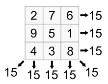

3-by-3 magic square

A magic square is a square table of positive integers, arranged such that every row sum, every column sum, and every diagonal sum are equal. For a 3-by-3 square this total is 15.

Write a function that takes a 3-by-3 integer matrix, returns TRUE if the matrix is a magic square, and FALSE otherwise.

is.magic <- function(m){
    if( !(nrow(m) == 3 & ncol(m) == 3)) {
        print("The matrix must be 3-by-3.")
        return()
    }
    all(
    rowSums(m) == rep(15,3),
    colSums(m) == rep(15,3),
    sum(diag(m)) == 15,
    m[1,3]+m[2,2]+m[3,1] == 15
    )
}

is.magic( matrix(c(2,9,4,7,5,3,6,1,8), nrow = 3) )  # TRUE

[1] TRUE

is.magic( matrix(1:9, ncol = 3)) # FALSE

[1] FALSE

is.magic( matrix(1:12, ncol = 3)) # error message

[1] "The matrix must be 3-by-3."

NULL

Random search for a magic square

Generate many random 3-by-3 matrices with entries from 1 to 9, and try to find magic squares.

for (i in 1:1e5) {
    m <- matrix(sample(1:9),nrow=3)
    if (is.magic(m))
        print(m)
}

     [,1] [,2] [,3]
[1,]    6    7    2
[2,]    1    5    9
[3,]    8    3    4
     [,1] [,2] [,3]
[1,]    4    9    2
[2,]    3    5    7
[3,]    8    1    6
     [,1] [,2] [,3]
[1,]    4    9    2
[2,]    3    5    7
[3,]    8    1    6