8 Repetition structures

Repetition (also known as “loops”) are another fundamental structure of all programming languages.

Repetition, like decision, requires a condition to execute a block of code. However, unlike decision, at the end of the block it checks the condition again. If the condition still holds, the block is executed again.

flowchart
  B[Code body] --> C{Condition}
  C -- True --> D[Execute if True]
  D --> C
  C -- False --> E[Code body]

Repetition flow diagram.

The while loop

Simple example: Print the squares of 1, 2, … 10.

Without loops, it would be cumbersome:

i <- 1
cat(i,i^2,"\n")

1 1

i <- i+1
cat(i,i^2, "\n")

2 4

i <- i+1
cat(i,i^2, "\n")

3 9

With loops, it is shorter and more flexible:

i <- 1 # initialization
while (i<=10) {  # condition
    cat(i,i^2,"\n")
    i <- i+1  # update
}

General structure of the `while` loop

<initialization>
while( <condition> ) {
    <statements>
    <update variables>
}

<condition> is a Boolean expression, usually involving existing variables.
If <condition> is true the block is executed (this is called one iteration).
When the block is completed, the condition is reevaluated and the block is re-executed if necessary.

Updating the variables

In general, we want the condition to become false eventually, otherwise the loop never ends.
The variables of the program must be updated within the block to ensure that.

i <- 1 # initialization
while (i<=10) {  # condition
    cat(i,i^2,"\n")
    i <- i+1  # update
}

Example

Find the sum of elements in a vector

Without a loop:

mydata <- c(-1,4,2,5,1,4,6,2,0)
total <- 0
i <- 1
total <- total + mydata[i]
i <- i+1
total <- total + mydata[i]
i <- i+1
total <- total + mydata[i]
#...

With a loop

mydata <- c(-1,4,2,5,1,4,6,2,0)
total <- 0
i <- 1
while (i<=length(mydata)){
    total <- total + mydata[i]
    cat(i, mydata[i], total, "\n")
    i <- i + 1
}

total

[1] 23

Example

Find the maximum element in a vector

mydata <- c(1,4,2,5,1,4,6,2,0,7,3,1)
largest <- mydata[1]
i <- 2
while (i<=length(mydata)){
    if(mydata[i]>largest)
        largest <- mydata[i]
    i <- i + 1
}
largest

[1] 7

The for loop

Alternative to while that does not take a Boolean condition.
The for statement takes elements from a vector one by one, and runs the loop body with the current element.
The loop terminates when the last element is used.

for(i in c(2,-1,5,3,7)) {
    cat(i,i^2,"\n")
}

In many cases for is simpler than while, especially when you need to iterate over the elements of a vector.

Example: Add up the elements in a vector with for:

mydata <- c(-1,4,2,5,1,4,6,2,0)
total <- 0
for (d in mydata)
    total <- total + d
total

[1] 23

The line for(d in mydata) means that d first gets mydata[1], then mydata[2], etc, until all the elements in mydata are used up.

Find the maximum value in a vector with a for loop.

mydata <- c(1,4,2,5,1,4,6,2,0)
largest <- mydata[1]
for(d in mydata) 
    if(d>largest) 
        largest <- d
largest

[1] 6

Note that by using for you don’t need to keep track of the element index. This is OK if you are interested in the element values only, but it might not work if the element’s location is relevant.

Example: Find the index of the maximum value in a vector.

mydata <- c(1,4,2,5,1,4,6,2,0)
largest <- mydata[1]
largest_index <- 1
i <- 2
while (i<=length(mydata)){
    if(mydata[i]>largest){
        largest_index <- i
        largest <- mydata[i]
    }
    i <- i + 1
}

cat(largest_index, largest)

7 6

Rewrite this as a function

getmax <- function(x) {
    largest <- x[1]
    largest_index <- 1
    i <- 2
    while (i<=length(x)){
        if(x[i]>largest){
            largest_index <- i
            largest <- x[i]
        }
        i <- i + 1
    }
    c(largest_index, largest)
}
getmax(mydata)

[1] 7 6

The `break` statement

When the program encounters a break statement, it terminates the loop. The remainder of the block is skipped over.

i <- 1
while(i<=10){
    if(i==7)
        break
    cat("i =",i,"\n")
    i <- i+1
}

i = 1 
i = 2 
i = 3 
i = 4 
i = 5 
i = 6

cat("Goodbye")

Goodbye

Same with a for loop

for(i in 1:10){
    if (i==7)
        break
    cat("i =",i,"\n")
}

i = 1 
i = 2 
i = 3 
i = 4 
i = 5 
i = 6

Example: Determine if a given number is prime

n <- 87659867241
prime <- TRUE # assume prime unless proven otherwise
i <- 2
while (i <= sqrt(n)){  # check only up to the square root of n
    if (n%%i == 0){
        prime <- FALSE
        break
    }
    i <- i+1
}
if (!prime) cat(n,"is not prime;",i,"divides it.")

87659867241 is not prime; 3 divides it.

Rewrite this as a function

isprime <- function(n) {
    prime <- TRUE # assume prime unless proven otherwise
    i <- 2
    while (i*i <= n){  # check only up to the square root of n
        if (n%%i == 0){
            prime <- FALSE
            break
        }
        i <- i+1
    }
    prime
}

isprime(87659867241)

[1] FALSE

The `next` statement

Takes the program flow to the beginning of the loop.
Skips over the remaining statements.

i<-0
while(i<=10){
    i <- i+1
    if( i%%3==0 )
        next
    cat(i, "")
}

1 2 4 5 7 8 10 11

Caution: If the update statement is located after next, the loop may not terminate.

i<-1
while(i<=10){
    if( i%%3==0 )
        next
    cat(i, "")
    i <- i+1
}

Example: Print the digits of a positive number

x <- 1764502
while (x>0){
    lastdig <- x%%10
    x <- floor( x/10 )
    cat(lastdig,"\n")
}

Collect into a vector:

x <- 1764502
v <- c()
while (x>0){
    v <- c(x%%10, v)
    x <- floor( x/10 )
}
v

[1] 1 7 6 4 5 0 2

The `repeat` loop

The repeat statement provides an infinite loop.
Does not take a test. To end the loop, use break.

i <- 1
repeat {
    i <- i + 3
    cat(i,"")
    if(i>10) break
}

4 7 10 13

The next statement works in the same way in repeat loops.

i <- -2
repeat {
    i <- i + 1
    if (i%%3==0) next
    cat(i,"")
    if(i>10) break
}

-1 1 2 4 5 7 8 10 11

Which type of loop should I use?

while is the most general one.
repeat is the same as while(TRUE).
for is more convenient when going over sequences such as vectors.

Nested loops

A loop body can contain anything, including other loops.

for (i in 1:4) {
    cat("i =",i,"\n")
    for (j in c(7,8,9))
        cat("   i+j =",i+j,"\n")
}

i = 1 
   i+j = 8 
   i+j = 9 
   i+j = 10 
i = 2 
   i+j = 9 
   i+j = 10 
   i+j = 11 
i = 3 
   i+j = 10 
   i+j = 11 
   i+j = 12 
i = 4 
   i+j = 11 
   i+j = 12 
   i+j = 13

Example: Print a triangle of stars with size 5.

*
**
***
****
*****

nlines <- 5
for (line in 1:nlines){
    for (col in 1:line)
        cat("*")
    cat("\n")
}

*
**
***
****
*****

Example: Simple bar chart

Given a vector x with positive integer entries, print x[l] stars for each line l.

x <- c(5,2,8,5,1,4,7,10,3)
for (line in 1:length(x)){
    for (col in 1:x[line])
        cat("*")
    cat("\n")
}

*****
**
********
*****
*
****
*******
**********
***

Example: All possible pairs from two vectors

Write a function that takes two vectors and prints products of all possible pairs from these vectors.

pair_product( 2:3, 7:9 )    
2 * 7 = 14 
2 * 8 = 16 
2 * 9 = 18 
3 * 7 = 21 
3 * 8 = 24 
3 * 9 = 27

In complicated problems, it is best to start with the simplest case and gradually add features.

First, take only two numbers and display their product:

a <- 2
b <- 7
cat(a, "*", b, "=", a*b, "\n")

2 * 7 = 14

Next, make one parameter a vector, and “wrap a loop” around cat().

a <- 2
b_vector <- c(7,3,8)
for (b in b_vector){
    cat(a, "*", b, "=", a*b, "\n")    
}

2 * 7 = 14 
2 * 3 = 6 
2 * 8 = 16

Finally, make the other factor a vector and wrap an outer loop around the existing loop.

pair_product <- function(a_vector, b_vector){
    for (a in a_vector){
        for (b in b_vector){
            cat(a, "*", b, "=", a*b, "\n")
        }
    }
}
pair_product(c(2,3,-1),c(7,3,8,5))

2 * 7 = 14 
2 * 3 = 6 
2 * 8 = 16 
2 * 5 = 10 
3 * 7 = 21 
3 * 3 = 9 
3 * 8 = 24 
3 * 5 = 15 
-1 * 7 = -7 
-1 * 3 = -3 
-1 * 8 = -8 
-1 * 5 = -5

Example: List Pythagorean triples

A Pythagorean triple consists of three integers a,b,c such that \(a^2 + b^2 = c^2\) holds. Let us determine all Pythagorean triplets such that \(a,b\leq 100\).

for (a in 1:100)
    for(b in b:100)
        for(c in b:142) # why 142? Max value of a^2+b^2
            if (a*a + b*b == c*c)
                cat(a,b,c,"\n")

75 100 125

The output above shows some triples such as 3 4 5 and 4 3 5, which are really not different. How do we remove such repetitions?

Performance of vectorized operations and loops

Many tasks involve applying looping over vector elements.
R has built-in vectorized functions for these tasks, but we can implement our own with loops.
Consider adding two vectors and assigning the result on a third:

x <- c(1,2,3)
y <- c(4,5,6)
z <- x + y
z

[1] 5 7 9

Alternative way by using a for loop

z <- vector(length=length(x))
for(i in 1:length(x))
    z[i] <- x[i] + y[i]
z

[1] 5 7 9

Let’s measure the time that the computer takes for each operation. We use large vectors so that we can see the time difference clearly.

x <- runif(1000000)
y <- runif(1000000)
system.time(z <- x+y) # Time taken by vectorized addition

   user  system elapsed 
  0.003   0.002   0.005

z <- vector(length=1000000)
system.time(for(i in 1:length(x)) z[i] <- x[i] + y[i]) # time taken by explicit loop.

   user  system elapsed 
  0.088   0.004   0.093

There is a large difference between execution times.
This is due to the implementation of R: The for() loop, the : operator, the index operator [ are all function calls, which slows the code.
Vectorized functions are written with C: They run fast.
When dealing with large data, use vectorized functions instead of a loop, whenever possible.

Further examples

Moving average

Moving averages are a way to reduce fluctuations in data. For example, the 2-element sample moving average of a vector \(v\) with \(n\) elements is defined as

\[ \left(\frac{v_1+v_2}{2},\frac{v_2+v_3}{2},\frac{v_3+v_4}{2}, \ldots, \frac{v_{n-1}+v_n}{2}\right)\]

Let’s generate some synthetic data with an upward trend and some random noise.

data <- cumsum(sample(c(-1,2),size = 100, replace=TRUE))
plot(data, type="l")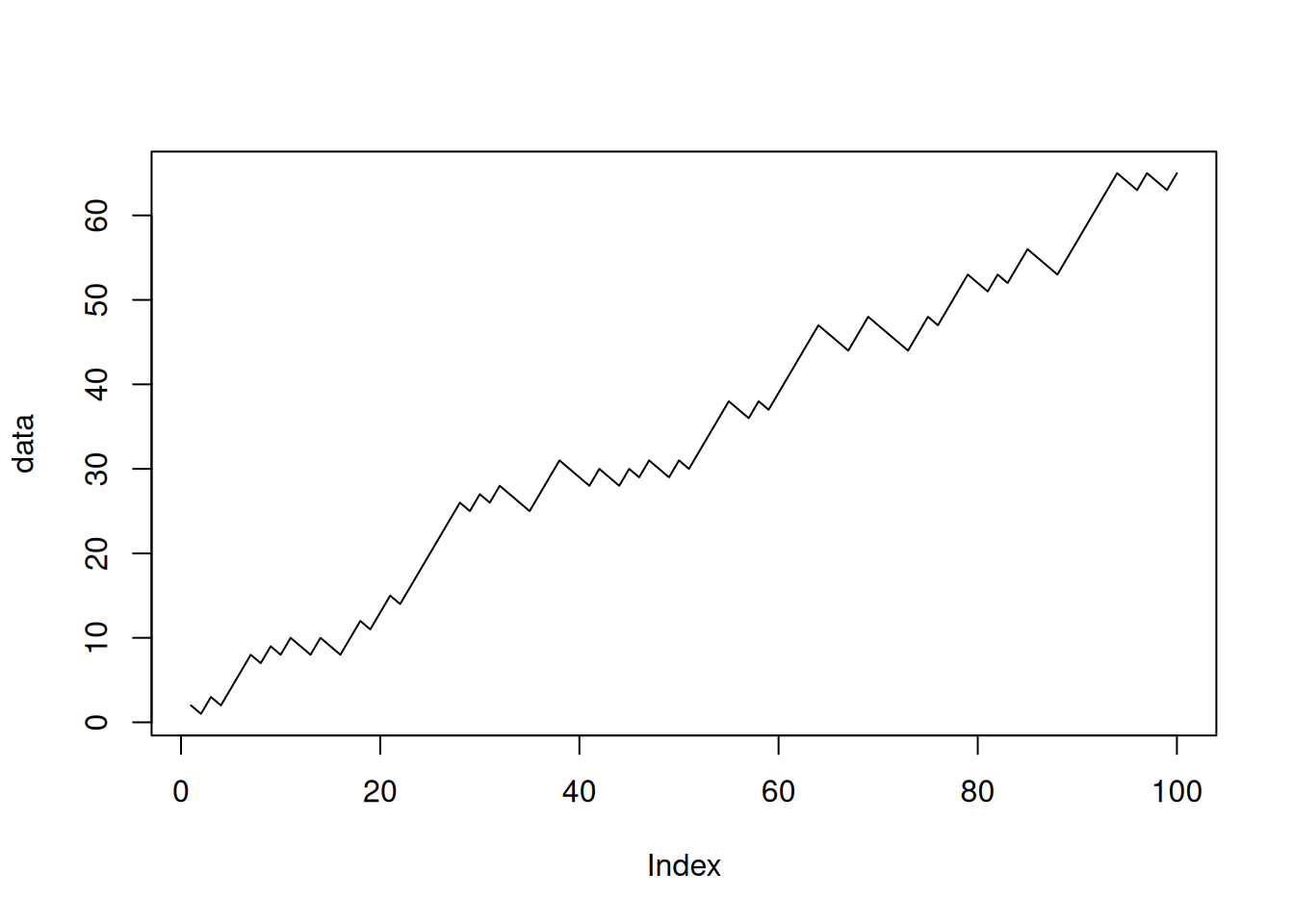

movav <- vector(length=length(data)-1)
for(i in 1:length(data)-1)
    movav[i] <- (data[i] + data[i+1])/2

plot(data, type="l")
lines(movav, col="red")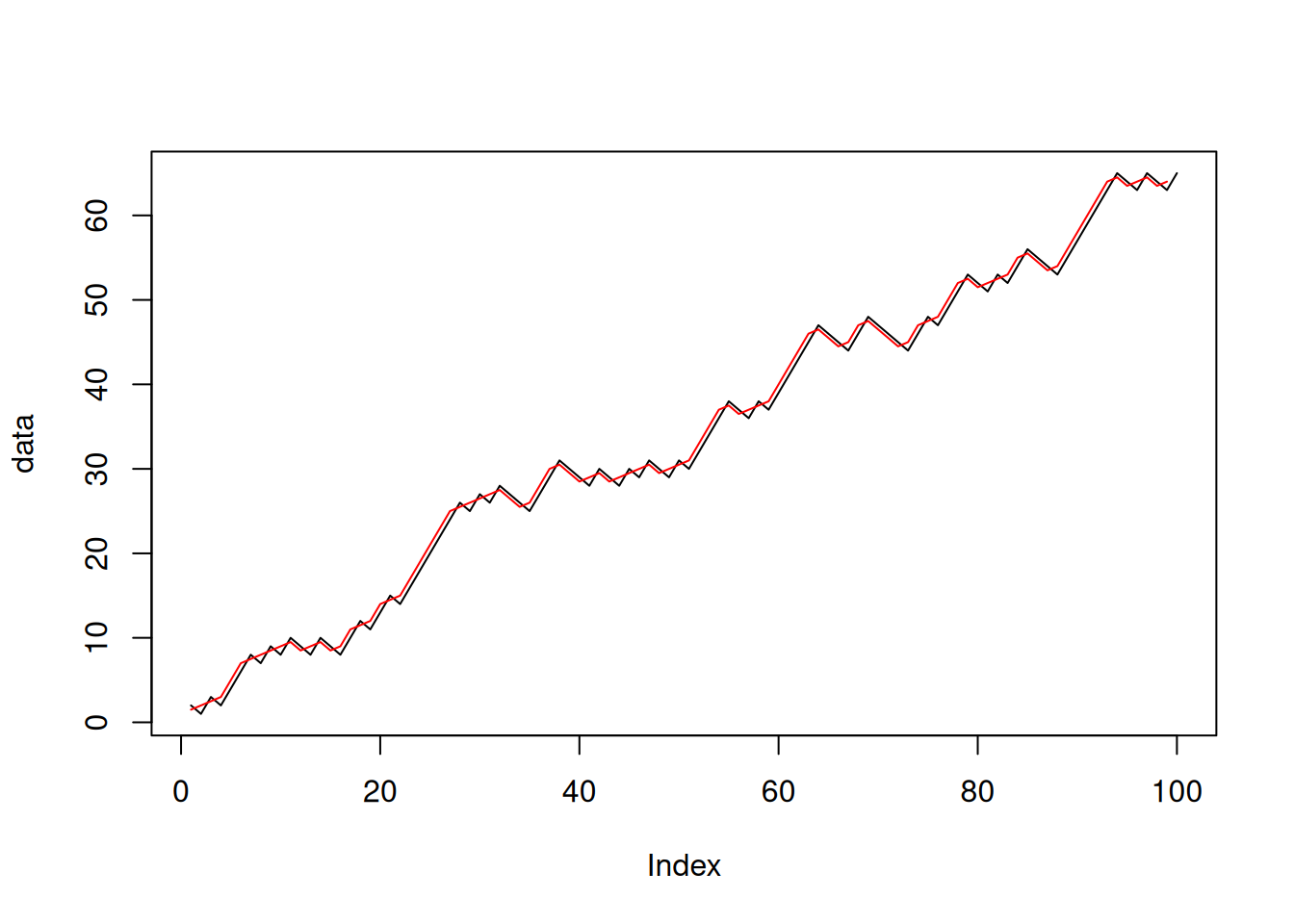

Implement this in vectorized form:

movav <- (data[1:length(data)-1] + data[2:length(data)])/2

Fibonacci sequence

A Fibonacci sequence starts with 1 and 1, and each new value is the sum of the two previous values. Formally: \[\begin{eqnarray} F_1 &=& 1\\ F_2 &=& 1\\ F_{n} &=& F_{n-1} + F_{n-2} \end{eqnarray}\]

Each number in this sequence is called a Fibonacci number. Let us write R code that displays the first 20 Fibonacci numbers.

f1 <- 1
f2 <- 1
for (i in 3:20){
    temp <- f1
    f1 <- f2
    f2 <- f2 + temp
    cat(f2,"\n")
}

Compound interest

account_balance <- 10000
interest_rate <- 0.1
years <- 10
balance_vec <- account_balance
for (y in 1:years){
    account_balance <- account_balance * (1+interest_rate)
    balance_vec <- c(balance_vec, account_balance)
    cat("After",y,"years your account balance is",account_balance,"\n")
}

After 1 years your account balance is 11000 
After 2 years your account balance is 12100 
After 3 years your account balance is 13310 
After 4 years your account balance is 14641 
After 5 years your account balance is 16105.1 
After 6 years your account balance is 17715.61 
After 7 years your account balance is 19487.17 
After 8 years your account balance is 21435.89 
After 9 years your account balance is 23579.48 
After 10 years your account balance is 25937.42

Series sum

Evaluate the sum \[\sum_{i=1}^{n} 2^{-i} = \frac{1}{2} + \frac{1}{4} +\ldots + \frac{1}{2^n}\] for given \(n\).

n <- 5
total <- 0
for (i in 1:n) {
    total <- total + 1/2^i
}
total

[1] 0.96875

As \(n\rightarrow\infty\), the sum must approach 1. To see this, let us wrap another loop around the code to change n.

for (n in 2:20){
    total <- 0
    for (i in 1:n) {
        total <- total + 1/2^i
    }
    cat("n =",n,", series total =",total,"\n")
}

n = 2 , series total = 0.75 
n = 3 , series total = 0.875 
n = 4 , series total = 0.9375 
n = 5 , series total = 0.96875 
n = 6 , series total = 0.984375 
n = 7 , series total = 0.9921875 
n = 8 , series total = 0.9960938 
n = 9 , series total = 0.9980469 
n = 10 , series total = 0.9990234 
n = 11 , series total = 0.9995117 
n = 12 , series total = 0.9997559 
n = 13 , series total = 0.9998779 
n = 14 , series total = 0.999939 
n = 15 , series total = 0.9999695 
n = 16 , series total = 0.9999847 
n = 17 , series total = 0.9999924 
n = 18 , series total = 0.9999962 
n = 19 , series total = 0.9999981 
n = 20 , series total = 0.999999

Exercises

Implement `sum` and `cumsum`

Implement the sum() and cumsum() functions using R’s loop structures. Test your functions with some simple cases to ensure that they work correctly. Using random vectors of size 1,000,000 as input, compare their speed with the built-in versions.

Digits of a number

Write a function digits(x) that takes a positive integer and returns a vector of its digits. For example, digits(0667230) should return the vector (6,6,7,2,3,0).

Digital sums

Write a function named digitsum which takes a positive integer and returns the sum of digits (the “digital sum”) of the input. For example, the function call digitsum(35274) should return 3+5+2+7+4=21.

Using this function, find the number between 1 and 1 million that has the largest digital sum.

Migration

Currently there are 1,000,000 inhabitants in city A, and 500,000 in city B. Each year, 2% of people in city A move to city B, and 3% of people in city A move to city B. The intrinsic growth rate of both cities is 1% (i.e., the growth in the absence of any migration).

Plot the population of both cities for the next 20 years.

Collatz numbers

The Collatz sequence is defined as follows:

Start with any positive integer \(n\).
If \(n\) is even, set \(n \leftarrow n/2\)
If \(n\) is odd, set \(n \leftarrow 3n+1\)
If \(n=1\), stop.

For example, starting with 10, the Collatz sequence is 10, 5, 16, 8, 4, 2, 1. The number of steps required to reach 1 is 6.

It is believed that for any starting point the sequence ends with 1. However, this is not proven.

Write a function collatzlen(n) that returns the number of steps required to go from n to 1 in a Collatz sequence. For example, collatzlen(10) should return 6.
Plot the Collatz sequence length for \(n\) going from 2 to 100.
For which starting value between 100 and 200 does the Collatz sequence have the largest length?

The while loop

General structure of the while loop

Updating the variables

Example

Example

The for loop

The break statement

The next statement

The repeat loop

Nested loops

Performance of vectorized operations and loops

Further examples

Moving average

Fibonacci sequence

Compound interest

Series sum

Exercises

Implement sum and cumsum

Digits of a number

Digital sums

Migration

Collatz numbers

General structure of the `while` loop

The `break` statement

The `next` statement

The `repeat` loop

Implement `sum` and `cumsum`