12  Factors and categories

Consider the following data table:

Name	Gender	Month of Birth
Can	Male	January
Cem	Male	July
Hande	Female	May
Mehmet	Male	May
Deniz	Female	February
Kemal	Male	July
Derya	Female	May
Fatma	Female	April

All values in this data are strings. However, Gender and Month of Birth take only a limited set of values. They are categorical variables.

A categorical variable (or, a factor) can take one of predetermined, discrete values. Day of the week, month of the year, shirt size are categorical variables.

A single value of a categorical variable is called a level, such as “Monday”, “December”, or “XL”

Create factor variables

First, let’s generate vectors to hold the relevant data.

name <- c("Can","Cem","Hande","Mehmet","Deniz","Kemal","Derya","Fatma")
gender <- c("Male","Male","Female","Male","Female","Male","Female","Female")
mode(gender)

[1] "character"

These vectors are of “character” type. We can convert the gender vector to a factor variable using the factor() function.

gender_fac <- factor(gender)
gender_fac

[1] Male   Male   Female Male   Female Male   Female Female
Levels: Female Male

mode(gender_fac)

[1] "numeric"

The mode() call on the factor variable returns numeric, because internally the levels are stored as integers 1,2,3… This fact makes it possible to add, remove, or rename levels.

Getting the levels of a factor

The factor vector has an additional attribute, the levels information.

Get the vector of levels:

levels(gender_fac)

[1] "Female" "Male"  

Get the number of levels:

nlevels(gender_fac)

[1] 2

Common R functions handle factors in specialized ways:

summary(gender)  # character vector

   Length     Class      Mode 
        8 character character 

summary(gender_fac) # factor

Female   Male 
     4      4 

One can change the level names easily using an assignment to the levels() function.

levels(gender_fac) <- c("F","M")
gender_fac

[1] M M F M F M F F
Levels: F M

Indexing and subsetting

Elements of factor-valued vectors are indexed in the same way as any other vector.

gender_fac[2:5]

[1] M F M F
Levels: F M

gender_fac[c(3,5,7:8)]

[1] F F F F
Levels: F M

Note that the last result is composed of only F levels. However, the factor object still stores the the full set of levels F and M.

Filtering with factors

Our factor-valued vector:

gender_fac

[1] M M F M F M F F
Levels: F M

As usual, the equality check returns a Boolean vector:

gender_fac=="M"

[1]  TRUE  TRUE FALSE  TRUE FALSE  TRUE FALSE FALSE

Among the name vector, select elements with corresponding gender "M".

name[gender_fac=="M"]

[1] "Can"    "Cem"    "Mehmet" "Kemal" 

Removing categories

Sometimes we may want to remove one level in a category.

As an example, consider the following factor, where the level "Female" is misspelled twice as "female":

gender_fac <- factor(c("Male","Male","Female","Male","female","Male","female","Female"))
gender_fac

[1] Male   Male   Female Male   female Male   female Female
Levels: female Female Male

The resulting factor has three levels, but actually "female" and "Female" should be the same the same. Let’s fix this by overwriting all occurrences of "female" with "Female".

gender_fac[gender_fac=="female"] <- "Female"
gender_fac

[1] Male   Male   Female Male   Female Male   Female Female
Levels: female Female Male

However, the levels attribute still lists the invalid "female" category. To remove it, we use the droplevels() function. It removes all levels for which there are no entries.

gender_fac <- droplevels(gender_fac)
gender_fac

[1] Male   Male   Female Male   Female Male   Female Female
Levels: Female Male

Nominal and ordinal factors

Consider the following table again:

Name	Gender	Month of Birth
Can	Male	January
Cem	Male	July
Hande	Female	May
Mehmet	Male	May
Deniz	Female	February
Kemal	Male	July
Derya	Female	May
Fatma	Female	April

gender is an example of a nominal factor: There is no inherent order between levels. We cannot say whether “Male” is greater than “Female” or not.

On the other hand, month of birth information is an ordinal factor: Months have an inherent order, so it makes sense to say that “January” < “February”.

Suppose we use a vector to store the observed month-of-birth (MOB) data.

mob <- c("January","July","May","May","February","July","May","April")

There are two problems with this vector:

1. Only five unique months appear in it. Other possible levels of this factor are not represented.
2. It doesn’t reflect the natural order of the months. If you compare January and February to see which is greater, you get:

mob[1] < mob[5]

[1] FALSE

because the less-than operator compares with alphabetical order only.

Defining the data as a factor object solves both problems, if we set the levels properly. This can be done as follows:

months <- c("January","February","March","April","May",
            "June","July","August","September","October","November","December")
mob_fac <- factor(mob, levels=months, ordered=TRUE)
mob_fac

[1] January  July     May      May      February July     May      April   
12 Levels: January < February < March < April < May < June < ... < December

The ordered=TRUE setting ensures that this is an ordinal factor, and comparisons can be made in the same order levels are given.

mob_fac[1] < mob_fac[5]  # January < February

[1] TRUE

The summary() function gives a count of elements in each level.

summary(mob_fac)

  January  February     March     April       May      June      July    August 
        1         1         0         1         3         0         2         0 
September   October  November  December 
        0         0         0         0 

Combining factor objects

Earlier we have seen that combining two vectors into a single vector is done with the c() function:

x1 <- c(1,2,3,4)
x2 <- c(7,8,9)
c(x1, x2)

[1] 1 2 3 4 7 8 9

The same works with factor objects:

mob_fac

[1] January  July     May      May      February July     May      April   
12 Levels: January < February < March < April < May < June < ... < December

mob2 <- factor(c("April","March","May"), levels=months, ordered=TRUE)
mob2

[1] April March May  
12 Levels: January < February < March < April < May < June < ... < December

c(mob_fac, mob2)

 [1] January  July     May      May      February July     May      April   
 [9] April    March    May     
12 Levels: January < February < March < April < May < June < ... < December

Binning

Often, a continuous data is converted to a categorical variable. For example, age is converted to young/middle-aged/old, body size to small/medium/large, income to low/high.

Suppose we are given the following, numerical data:

x <- c(11, 18, 36, 74, 43, 81, 95, 64, 32, 51)

We want to categorize this data as small for values in [0, 30), medium for [30, 70), and high for [70, 100].

The notation [30,70) means that the value 30 belongs to this category, but 70 does not.

The cut() function generates a factor object from continuous values. The breaks parameter is used to specify the intervals.

cut(x, breaks=c(0, 30, 70, 100))

 [1] (0,30]   (0,30]   (30,70]  (70,100] (30,70]  (70,100] (70,100] (30,70] 
 [9] (30,70]  (30,70] 
Levels: (0,30] (30,70] (70,100]

However, note that the ends of the intervals are not as we want. The first value of the boundary in not included in the interval, but the second value is.

To fix this, we set the parameter right to FALSE.

cut(x, breaks=c(0, 30, 70, 100), right = F)

 [1] [0,30)   [0,30)   [30,70)  [70,100) [30,70)  [70,100) [70,100) [30,70) 
 [9] [30,70)  [30,70) 
Levels: [0,30) [30,70) [70,100)

But the last value 100 is excluded now. We can include it by setting the include.lowest parameter to TRUE.

cut(x, breaks = c(0, 30, 70, 100),
    right = F, include.lowest = T)

 [1] [0,30)   [0,30)   [30,70)  [70,100] [30,70)  [70,100] [70,100] [30,70) 
 [9] [30,70)  [30,70) 
Levels: [0,30) [30,70) [70,100]

Level names are automatically set. We can rename them with the labels parameter.

cut(x, breaks = c(0, 30, 70, 100), 
    right = F, include.lowest = T,
    labels = c("Low","Medium","High"))

 [1] Low    Low    Medium High   Medium High   High   Medium Medium Medium
Levels: Low Medium High

Factors and data frames

One of the built-in data sets in R is the mtcars data. We can see its first six lines with the head() function call:

head(mtcars)

                   mpg cyl disp  hp drat    wt  qsec vs am gear carb
Mazda RX4         21.0   6  160 110 3.90 2.620 16.46  0  1    4    4
Mazda RX4 Wag     21.0   6  160 110 3.90 2.875 17.02  0  1    4    4
Datsun 710        22.8   4  108  93 3.85 2.320 18.61  1  1    4    1
Hornet 4 Drive    21.4   6  258 110 3.08 3.215 19.44  1  0    3    1
Hornet Sportabout 18.7   8  360 175 3.15 3.440 17.02  0  0    3    2
Valiant           18.1   6  225 105 2.76 3.460 20.22  1  0    3    1

This is an old data set from 1974, collecting some features of 32 automobiles. For more information, use the command help(mtcars).

The summary() function returns the summary statistics for each numeric field.

summary(mtcars)

      mpg             cyl             disp             hp       
 Min.   :10.40   Min.   :4.000   Min.   : 71.1   Min.   : 52.0  
 1st Qu.:15.43   1st Qu.:4.000   1st Qu.:120.8   1st Qu.: 96.5  
 Median :19.20   Median :6.000   Median :196.3   Median :123.0  
 Mean   :20.09   Mean   :6.188   Mean   :230.7   Mean   :146.7  
 3rd Qu.:22.80   3rd Qu.:8.000   3rd Qu.:326.0   3rd Qu.:180.0  
 Max.   :33.90   Max.   :8.000   Max.   :472.0   Max.   :335.0  
      drat             wt             qsec             vs        
 Min.   :2.760   Min.   :1.513   Min.   :14.50   Min.   :0.0000  
 1st Qu.:3.080   1st Qu.:2.581   1st Qu.:16.89   1st Qu.:0.0000  
 Median :3.695   Median :3.325   Median :17.71   Median :0.0000  
 Mean   :3.597   Mean   :3.217   Mean   :17.85   Mean   :0.4375  
 3rd Qu.:3.920   3rd Qu.:3.610   3rd Qu.:18.90   3rd Qu.:1.0000  
 Max.   :4.930   Max.   :5.424   Max.   :22.90   Max.   :1.0000  
       am              gear            carb      
 Min.   :0.0000   Min.   :3.000   Min.   :1.000  
 1st Qu.:0.0000   1st Qu.:3.000   1st Qu.:2.000  
 Median :0.0000   Median :4.000   Median :2.000  
 Mean   :0.4062   Mean   :3.688   Mean   :2.812  
 3rd Qu.:1.0000   3rd Qu.:4.000   3rd Qu.:4.000  
 Max.   :1.0000   Max.   :5.000   Max.   :8.000  

Even though all data appears as numeric, some columns are actually categorical: "cyl" gives the number of cylinders in the engine, "vs" indicates if the car has a V-shaped engine (0) or a straight (0), "am" indicates if it has automatic transmission (0) or manual (1), "gear" is the number of forward gears, and "carb" is the number of carburetors.

If we convert these columns to factors, summary() and other R functions will give more relevant information about the data.

cyl, gear and carb are ordinal factors (can be ordered meaningfully), so we set ordered=TRUE for them.

mtcars$cyl <- factor(mtcars$cyl, ordered=TRUE)
mtcars$gear <- factor(mtcars$gear, ordered=TRUE)
mtcars$carb <- factor(mtcars$carb, ordered=TRUE)
mtcars$vs <- factor(mtcars$vs)
mtcars$am <- factor(mtcars$am)

Now we can use the summary() function to get the counts of categories in each factor field.

summary(mtcars)

      mpg        cyl         disp             hp             drat      
 Min.   :10.40   4:11   Min.   : 71.1   Min.   : 52.0   Min.   :2.760  
 1st Qu.:15.43   6: 7   1st Qu.:120.8   1st Qu.: 96.5   1st Qu.:3.080  
 Median :19.20   8:14   Median :196.3   Median :123.0   Median :3.695  
 Mean   :20.09          Mean   :230.7   Mean   :146.7   Mean   :3.597  
 3rd Qu.:22.80          3rd Qu.:326.0   3rd Qu.:180.0   3rd Qu.:3.920  
 Max.   :33.90          Max.   :472.0   Max.   :335.0   Max.   :4.930  
       wt             qsec       vs     am     gear   carb  
 Min.   :1.513   Min.   :14.50   0:18   0:19   3:15   1: 7  
 1st Qu.:2.581   1st Qu.:16.89   1:14   1:13   4:12   2:10  
 Median :3.325   Median :17.71                 5: 5   3: 3  
 Mean   :3.217   Mean   :17.85                        4:10  
 3rd Qu.:3.610   3rd Qu.:18.90                        6: 1  
 Max.   :5.424   Max.   :22.90                        8: 1  

The "vs" (V-shaped engine or straight) and "am" (Automatic or manual transmission) fields have level values 0 or 1.

levels(mtcars$am)

[1] "0" "1"

Let’s replace the level values with clearer labels.

levels(mtcars$vs) <- c("V-engine","Standard")
levels(mtcars$am) <- c("Automatic","Manual")

summary(mtcars)

      mpg        cyl         disp             hp             drat      
 Min.   :10.40   4:11   Min.   : 71.1   Min.   : 52.0   Min.   :2.760  
 1st Qu.:15.43   6: 7   1st Qu.:120.8   1st Qu.: 96.5   1st Qu.:3.080  
 Median :19.20   8:14   Median :196.3   Median :123.0   Median :3.695  
 Mean   :20.09          Mean   :230.7   Mean   :146.7   Mean   :3.597  
 3rd Qu.:22.80          3rd Qu.:326.0   3rd Qu.:180.0   3rd Qu.:3.920  
 Max.   :33.90          Max.   :472.0   Max.   :335.0   Max.   :4.930  
       wt             qsec              vs             am     gear   carb  
 Min.   :1.513   Min.   :14.50   V-engine:18   Automatic:19   3:15   1: 7  
 1st Qu.:2.581   1st Qu.:16.89   Standard:14   Manual   :13   4:12   2:10  
 Median :3.325   Median :17.71                                5: 5   3: 3  
 Mean   :3.217   Mean   :17.85                                       4:10  
 3rd Qu.:3.610   3rd Qu.:18.90                                       6: 1  
 Max.   :5.424   Max.   :22.90                                       8: 1  

Plotting factor variables

When given a factor variable, the plot() function displays a bar plot by default.

plot(mtcars$am)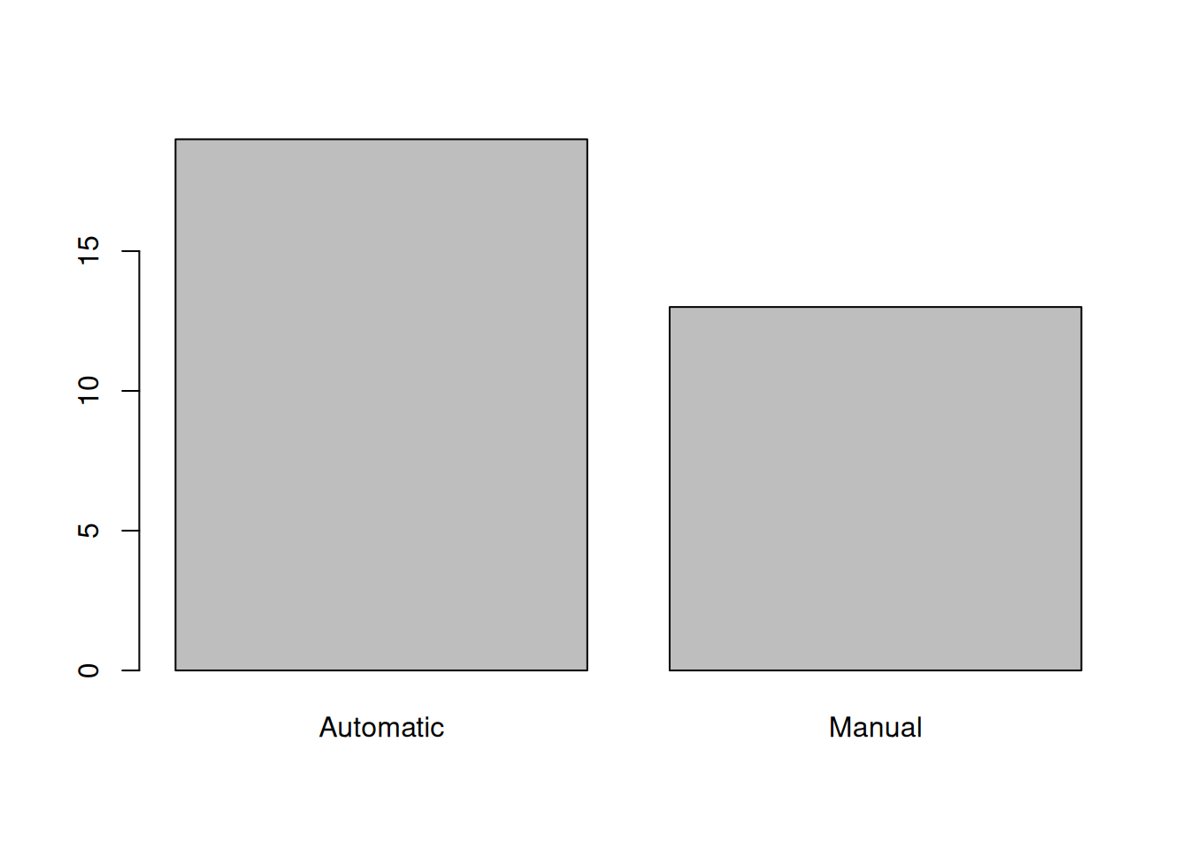

When the x-axis is categorical and the y-axis is numerical, a boxplot is displayed.

plot(x = mtcars$vs, y=mtcars$hp, ylab="Horse power")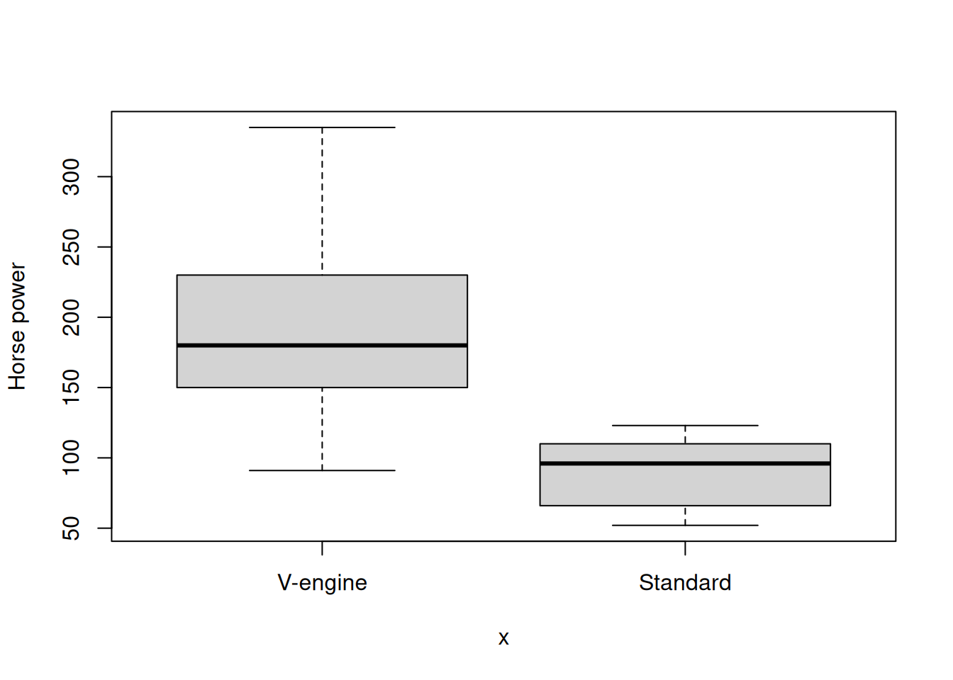

If both axes are categorical, a stacked bar plot is displayed.

plot(x = mtcars$vs, y=mtcars$gear, xlab="Engine type",ylab="Gear")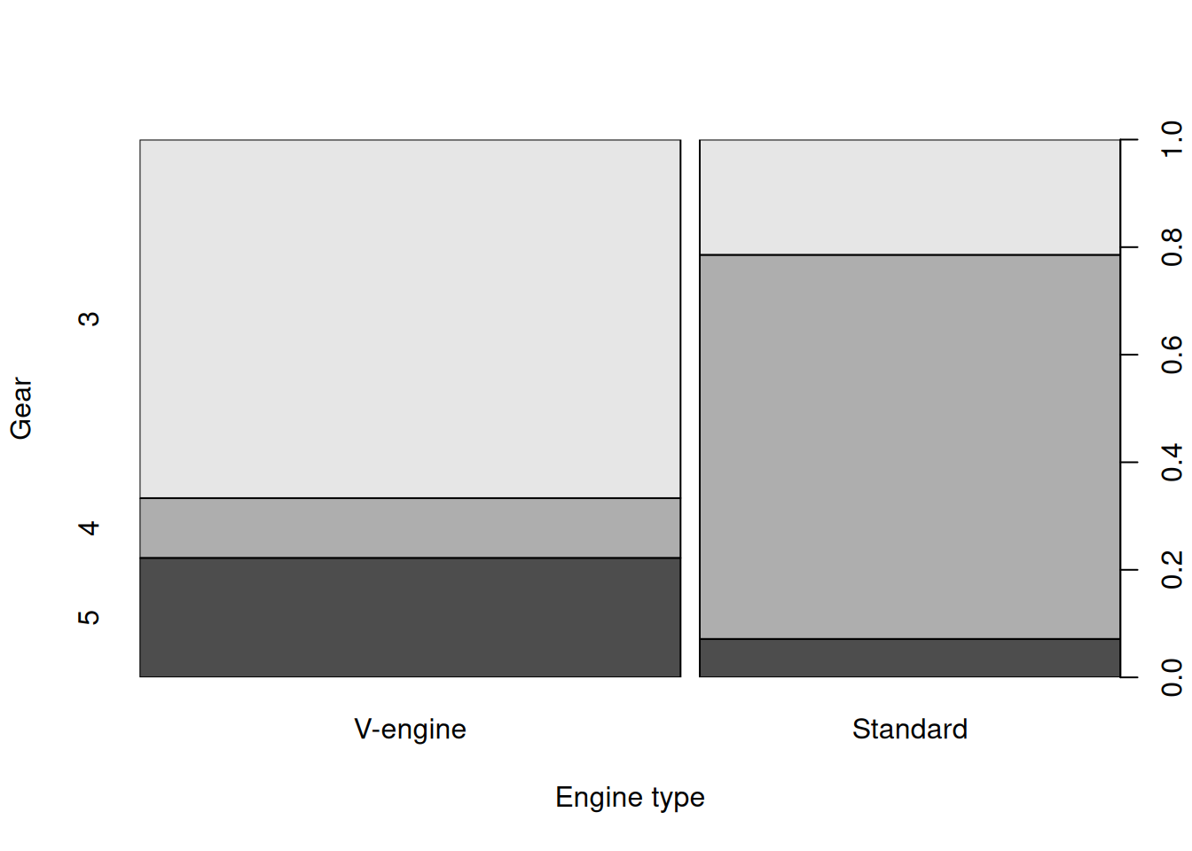

The table() function

The table() function can be used to return counts of elements in each level of a categorical variable.

affils <- c("R","D","D","R","U","D") # political party affiliations
table(affils)

affils
D R U 
3 2 1 

It can be used to create contingency tables, such as two-way tables:

table(mtcars$am, mtcars$vs)

           
            V-engine Standard
  Automatic       12        7
  Manual           6        7

Or three-way tables:

table(mtcars$am, mtcars$vs, mtcars$gear,
      dnn=c("Transmission","Engine","Gears"))

, , Gears = 3

            Engine
Transmission V-engine Standard
   Automatic       12        3
   Manual           0        0

, , Gears = 4

            Engine
Transmission V-engine Standard
   Automatic        0        4
   Manual           2        6

, , Gears = 5

            Engine
Transmission V-engine Standard
   Automatic        0        0
   Manual           4        1

The tapply() function

This is more general than table(). Both apply on groups broken by categories, but table() gives only the counts of these groups, while tapply() applies any function to the groups, such as the mean, median, or maximum.

The function call tapply(x, f, func) breaks the vector x by levels given in f and applies the function func on each subgroup.

Given the ages and party affiliations of a group of people, find the average age of people in every party:

ages <- c(25, 26, 55, 37, 21, 42) # ages of some people
affils <- c("R","D","D","R","U","D") # party affiliations of the same people
tapply(ages, affils, mean)

 D  R  U 
41 31 21 

Use the mtcars data again. Get the mean miles-per-gallon for each engine type.

tapply(mtcars$mpg, mtcars$vs, mean)

V-engine Standard 
16.61667 24.55714 

Get the mean miles-per-gallon again, broken by the engine type and transmission type.

tapply(mtcars$mpg, list(mtcars$vs, mtcars$am), mean)

         Automatic   Manual
V-engine  15.05000 19.75000
Standard  20.74286 28.37143

Finally, look at the built-in iris database, which stores measurements of sepals and petals of three species of iris flower.

head(iris)

  Sepal.Length Sepal.Width Petal.Length Petal.Width Species
1          5.1         3.5          1.4         0.2  setosa
2          4.9         3.0          1.4         0.2  setosa
3          4.7         3.2          1.3         0.2  setosa
4          4.6         3.1          1.5         0.2  setosa
5          5.0         3.6          1.4         0.2  setosa
6          5.4         3.9          1.7         0.4  setosa

Let’s get the mean sepal length of flowers, broken by the species:

tapply(iris$Sepal.Length, iris$Species, mean)

    setosa versicolor  virginica 
     5.006      5.936      6.588