6  Functions

A function is a piece of code that takes input arguments , performs a specific task, and returns its output.

We have seen quite a few built-in functions of R, such as c(), length(), runif(), mean(), or sum().

However, we are not limited to using built-in functions. We can define our own functions in order to complete one computing task.

A first example

Let us define a function that returns the square of a given number.

square <- function(x) {
    return(x^2)
}

We call the function by providing the input value as an argument. The function returns a value, which we can store in a variable.

foo <- square(3)
foo

[1] 9

If we type a function’s name and press Enter, we get back the definition of the function.

square

function (x) 
{
    return(x^2)
}

General syntax of function definition

A function can take any number of input arguments. It performs some computations in its body, and generates a return value. The returned value can be any R object (number, string, vector, list, dataframe, etc.)

<function_name> <- function([<argument_1>, <argument_2>, ...]) {
    <statements>
    return(<return_value>)
}

The return statement is optional. The function returns the value of the last expression in its block. So the function square() can also be defined as:

square <- function(x) {
    print(x)
    x^2
    }
sq3 <- square(3)

[1] 3

sq3

[1] 9

The job of the braces {} is to combine several statements into one.

As we have only one statement here, braces can be omitted and the function can be stated in one line.

square <- function(x) x^2
square(3)

[1] 9

Function arguments

A function can be defined with any number of arguments.

f <- function(x,y,z){
    return(x + y*z)
}
f(1,2,3)

[1] 7

It is possible to change the order of arguments by using the argument names explicitly:

f(z=3,x=1,y=2)

[1] 7

You can even omit some names, and the unnamed arguments will be matched in order.

f(z=3,1,2)

[1] 7

Return values

The return value of the function can be any R object, such as a number, a vector, a matrix, a list, etc.

sumdiff <- function(x,y){
    return( c(x+y, x-y) )
}

sumdiff(5,8)

[1] 13 -3

Functions returning functions

A function itself is an R object, therefore we can easily write functions that return functions.

Here is a function that returns a power function with any order we like:

powerfun <- function(p){
    return(function(y){return(y^p)})
}
# Alternatively:
# powerfun <- function(p) function(x) x^p

Now we can use this function to generate other functions:

sq <- powerfun(2)
cube <- powerfun(3)

sq

function (y) 
{
    return(y^p)
}
<environment: 0x5c68f1cc1cb8>

Evaluate functions with input value 5.

sq(5)

[1] 25

cube(5)

[1] 125

Functions with side effects

Sometimes we call a function not for its return value, but for its side effect, such as generating a plot.

plot_random_walk <- function(n){
    x <- cumsum(sample(c(-1,1), n, replace=TRUE))
    plot(x, type="o", xlab="step number", ylab="Distance from origin")
    title("A random walk")
}

set.seed(7652)
plot_random_walk(100)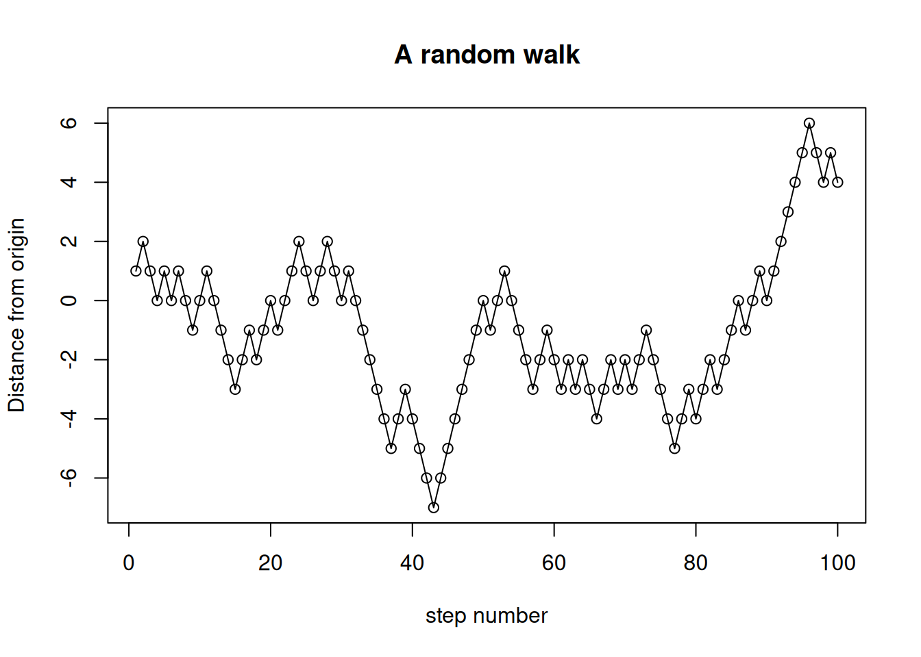

Vectorization of functions

The simple function square() defined above happens to work with vector arguments without any modification, because the returned statement x^2 is valid for both numbers and vectors.

square <- function(x) x^2
square(c(1,2,3,4,5))

[1]  1  4  9 16 25

However, functions are not always applicable with vector arguments as they are. For example, a function that returns the sum of integers from 1 up to its argument value:

addupto <- function(n) sum(1:n)
addupto(10)

[1] 55

When we call this function with a vector argument, only the first element is taken, and a warning message is issued

addupto(c(10,20)) # Internally it tries sum(1:c(10,20))

Warning in 1:n: numerical expression has 2 elements: only the first used

[1] 55

If you want this function to work with vector input, the preferred way in R is to use the built-in sapply function, which maps a function on each element of a vector.

sapply(c(10,20, 30, 40, 50), addupto)

[1]   55  210  465  820 1275

Default arguments

When you define a function, you can set some of the arguments to default values. Then you don’t have to specify them at each call.

f <- function(capital, interest_rate=0.1) {
    capital * (1+interest_rate)
}

Without specifying the interest_rate value, 0.1 is assumed.

f(1000)

[1] 1100

But if you want to change it, you can provide it as an extra argument.

f(1000, 0.2)

[1] 1200

Calling the function with argument names is usually clearer for the reader.

f(capital = 1000, interest_rate = 0.2)

[1] 1200

You can change the order of the arguments when you use argument names.

f(interest_rate=0.2, capital=1000)

[1] 1200

Scope of variables

• The value of a variable defined outside a function (a global variable) can be seen inside a function.
• However, a variable defined inside a function block is not recognized outside of it.
• We say that the scope of the variable b is limited to the function f().

a <- 5 # a global variable

f <- function(){
    b <- 10 # a local variable
    cat("inside f(): a =",a,"b =",b,"\n")
}

f()

inside f(): a = 5 b = 10 

cat("outside f(): a =",a," ")

outside f(): a = 5  

cat("b =",b)  # raises an error

Error: object 'b' not found

A local variable temporarily overrides a global variable with the same name.

a <- 5 # a global variable
cat("before f(): a =",a,"\n")

before f(): a = 5 

f <- function(){
    a <- 10 # a local variable
    cat("inside f(): a =",a,"\n")
}

f()

inside f(): a = 10 

cat("after f(): a =",a)

after f(): a = 5

Assigning values to upper-level variables

Although the values of variables defined in upper levels are available in lower levels, they cannot be modified in a lower level, because an assignment will create only a local variable with the same name.

Using the superassignment operator <<- it is possible to assign to a variable in the higher level.

a <- 5
cat("before f(): a =",a,"\n")

before f(): a = 5 

f <- function(){
    a <<- 10
    cat("inside f(): a =",a,"\n")
}

f()

inside f(): a = 10 

cat("after f(): a =",a)

after f(): a = 10

However, this is not recommended in general. It cause some subtle errors that are difficult to find. You almost never need this.

To modify a global variable, the most transparent way is to assign the function output to it explicitly.

a <- 5
cat("before f(): a =",a,"\n")

before f(): a = 5 

f <- function(x) {x+5}
a <- f(a)
cat("after f(): a =",a)

after f(): a = 10

Unspecified arguments with ...

Some functions take an unlimited number of arguments, e.g. c().

c(1,2,3)

[1] 1 2 3

c(4,2,6,1,3,5,1)

[1] 4 2 6 1 3 5 1

The c() function is defined with an ellipsis (three dots) as the argument list.

help(c)

Ellipsis has two use cases:

• Write a function that takes any number of arguments (like c() or sum()).
• Pass some arguments to another function, called inside the current function

Let’s modify our function for generating and plotting a random walk. It accepts some unspecified arguments represented with the ellipsis, and passes them to plot()

plot_random_walk <- function(n, ...){
    x <- cumsum(sample(c(-1,1), n, replace=TRUE))
    plot(x, type="o", ...)
} 

We can then call the function by specifying only the number of points:

options(repr.plot.width=10, repr.plot.height=4)
plot_random_walk(100)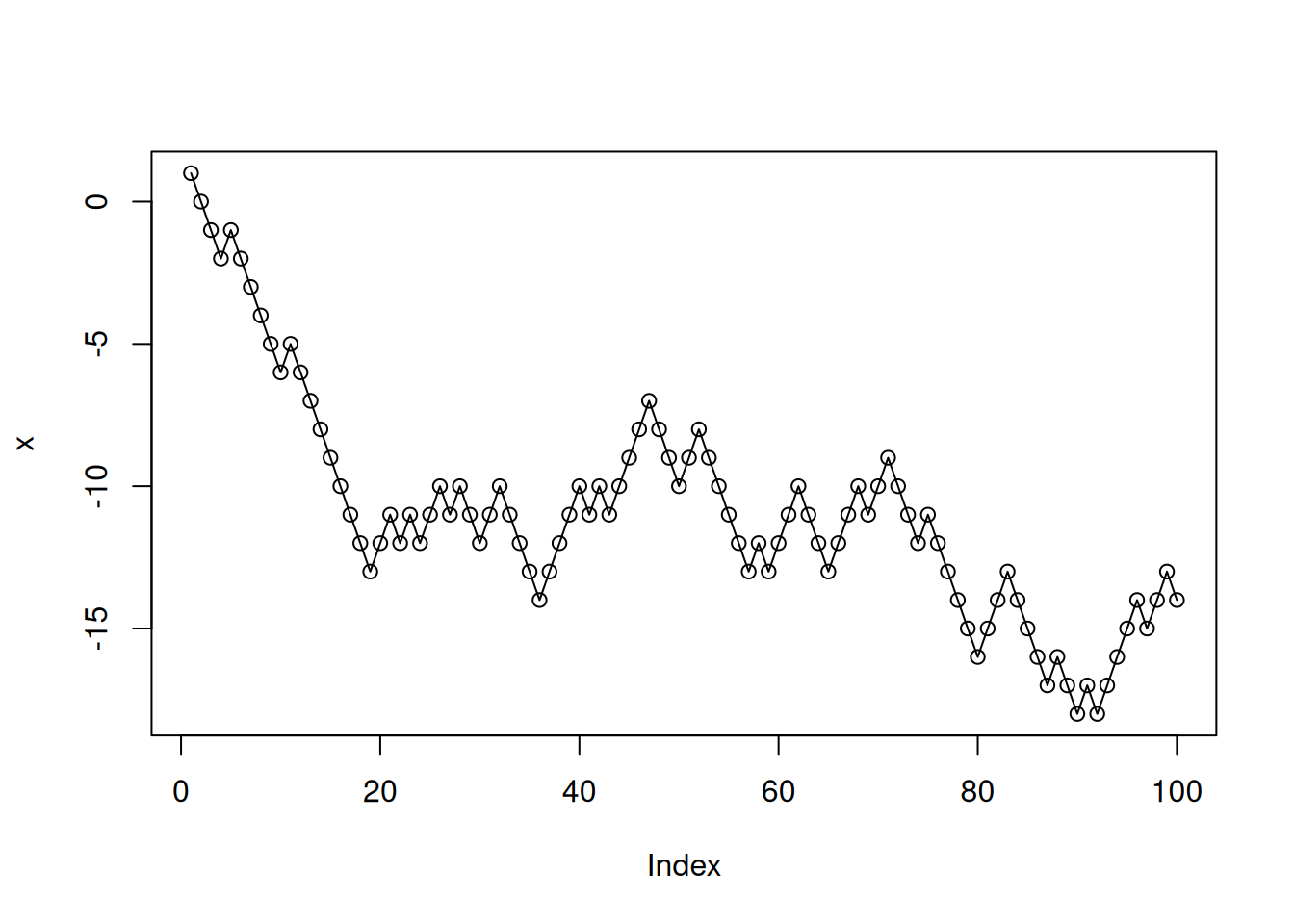

or by specifying plot parameters:

plot_random_walk(100, 
                 pch=4, 
                 col="red", 
                 main="A random walk", 
                 xlab="step number", 
                 ylab="displacement")

The arguments passed with the ellipsis can be converted to a vector, so we can process them inside the function.

diff <- function(...) {
    # returns the difference between the first and the last argument
    arguments <- c(...)
    cat("Number of arguments = ",length(arguments))
    arguments[length(arguments)] - arguments[1] # last argument minus first argument
}
diff(1,4,2)

Number of arguments =  3

[1] 1

diff(1,4,2,6,3,1)

Number of arguments =  6

[1] 0

Ellipsis arguments can have arbitrary names, and can be converted to a list object (more on lists later).

f <- function(...){
    args <- list(...)
    print(args)
}
f(a=1, b=3, foo=7654)

$a
[1] 1

$b
[1] 3

$foo
[1] 7654

Exercises

Write a function with the name FtoC that takes a temperature measurement in degrees Fahrenheit, and returns the equivalent value in degrees Celsius. Make sure that your function works with vector input, too.

---

Write a function with the name bmi that takes two arguments, height and weight, and returns the body-mass index calculated with these argument values. The function should work with vector input, too.

---

Write a function named range that takes a vector of numbers, and returns the difference between its minimum and the maximum elements. Test your function with some randomly-generated vectors.

---