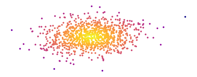
Suppose you have a set of data, which is concentrated around some mode value, as usual. The farther out you go, the fewer points you have. In other words, large deviations from the mode is unlikely. The larger, the unlikelier. (A very small value may count as a large deviation in the other direction, depending on the distribution.)
You might want to have a numerical estimate of how unlikely these outliers are. That is, what is the probability to see such a big deviation, or bigger?1
1 This is called the survival function. \(S_X(x) := \mathrm{Pr}(X>x)\)
This probability would be useful for interpreting your results, or for detecting an anomaly. If you find a once-a-year data point occurring two or three times within a week, you might want to investigate.
Once is happenstance. Twice is coincidence. Three times, it’s enemy action. – Ian Fleming, “Goldfinger”
However, estimating the probability of rare events is tricky. True, if you know the parent distribution of the data, you can easily use the cumulative distribution function2 to calculate that probability. But, with real data, we don’t know the parent distribution with certainty.
2 A.k.a. CDF, defined as \(F_X(x)=\mathrm{Pr}(X\leq x)=1-S_X(x)\)
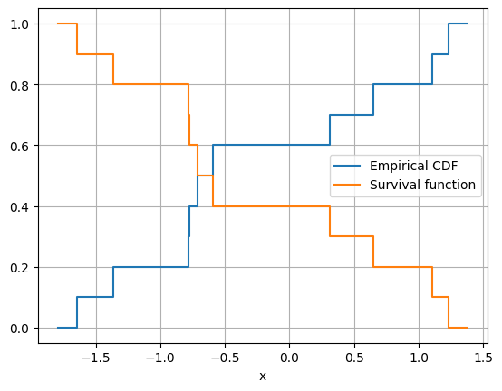
Without a model of the parent distribution, we can use the empirical distribution function. This is simple enough: Just count the fraction of your data points below a value. However, the empirical distribution function will not help with a new large value. The survival function for this new value will just be zero, simply because the data’s larger than any we have seen so far.
We can use Extreme Value Theory to estimate the tail probabilities based on empirical data only. Specifically, the theory states that data points larger than a threshold are distributed, approximately, as the Generalized Pareto distribution.
Let’s see how this theory is applied.
The Peak-Over-Threshold approach
Suppose that we have a set of observations \(\lbrace x_1, x_2, \ldots, x_n\rbrace\). The values \(x_i\) are realizations of a random variable \(X\), which is distributed according to an unknown cumulative distribution function \(F_X(x) = \mathrm{Pr}( X<x)\). In practice we do not know the parent distribution \(F_X(x)\).

If we are mainly interested in the behaviour of rare values, the Peaks-Over-Threshold method provides a good fit to the distribution’s tail. The idea is to select data points above a given threshold \(u\) and build a conditional probability distribution with them.
We first define the variable \(Y\equiv X-u\), called the excess, which gives how much \(X\) exceeds \(u\).
Also define the conditional excess distribution function \(F_{Y|u}(y)\) as:
\[\begin{equation} F_{Y|u}(y) = \mathrm{Pr}(X-u \leq y | X>u). \end{equation}\]
The condition is necessary because we assume that the variable \(X\) is larger than the threshold \(u\).
Using the definition of conditional probability, this can be rewritten as
\[\begin{align} F_{Y|u}(y) &=& \mathrm{Pr}(X \leq y+u | X>u) \\ &=& \frac{\mathrm{Pr}(X \leq y+u , X>u)}{\mathrm{Pr}(X>u)}\\ &=& \frac{F_X(u+y) - F_X(u)}{1-F_X(u)}\\ &=& \frac{F_X(x) - F_X(u)}{1-F_X(u)} \end{align}\]
Solving for \(F_X(x)\), we get:
\[\begin{equation} F_X(x) = \left(1-F_X(u)\right)F_{Y|u}(y) + F_X(u) \end{equation}\]
We estimate \(F_X(u)\) using the data directly, as the fraction of all observations less than or equal to \(u\):
\[\begin{equation} \hat{F}_X(u) = \frac{n-N_u}{n} \end{equation}\] where \(n\) is the number of all observations and \(N_u\) is the number of observations equal or larger than \(u\).
The remaining piece is \(F_{Y|u}(y)\). To estimate it, we use the Pickands-Balkema-de Haan theorem from extreme value theory. The theorem states that, for large \(u\), \(F_{Y|u}\) is well-approximated by the Generalized Pareto Distribution \(G_{k,\sigma}(y)\), where \[\begin{equation} \lim_{u\rightarrow\infty} F_{Y|u}(y) = G_{k,\sigma}(y) = \begin{cases} 1 - \left(1 + \frac{ky}{\sigma}\right)^{-1/k} & \text{if } k\neq 0 \\ 1 - \mathrm{e}^{-y/\sigma} & \text{if } k=0 \\ \end{cases} \end{equation}\] Here \(\sigma > 0\) is the scaling parameter and \(k\) is the shape parameter, also known as the tail index.
Plugging in the Pickands-Balkema-de Haan approximation, we get an estimation for the distribution \(F_X(x)\) for large \(u\) and \(x>u\): \[\begin{equation} \hat{F}_X(x) = \left(1 - \frac{n-N_u}{n}\right)G_{k,\sigma}(x-u) + \frac{n-N_u}{n} \end{equation}\] Finally, after simplification, we get the tail approximation for the unknown distribution \(F_X(x)\): \[\begin{equation} \hat{F}_X(x) = 1 + \frac{N_u}{n}\left(G_{k,\sigma}(x-u)-1\right). \end{equation}\] The parameters \(N_u\), \(k\) and \(\sigma\) should be estimated from given data \(\lbrace x_1, x_2, \ldots, x_n\rbrace\) and fixed \(u\).
The approximation is gets better as the threshold \(u\) increases. However, if we set the threshold too large, there will be an insufficient amount of data to fit the distribution parameters. To balance these requirements, we set \(u\) such that 10% of data is above it.
Implementation
Here we write a Python implementation of the this cumulative distribution function. Up to the threshold \(u\), the function is equal to the empirical distribution function. Above the threshold, it returns the tail approximation.
We do not use the threshold \(u\) directly, but we set a fixed percentile \(q\) (e.g. \(q=0.9\)). The two are related with the empirical CDF as \(q = F_n(u)\). Using the percentile makes the implementation easier: Tail points are simply selected as the \(q\)-quantile of the data.
To estimate the parameters of the Generalized Pareto Distribution, we use the method implemented in Scipy. Internally, SciPy uses maximum-likelihood estimation to infer the parameters.
import numpy as np
from scipy import stats

def ecdf_tail_approx(x, q=0.9):
    """Return the empirical cumulative distribution function (CDF)
    where the tail has the Generalized Pareto form.

    Parameters
    ----------
    x : numpy array
        The input data.
    q : float, optional. Default: 0.9
        The quantile threshold for switching to the conditional
        excess distribution function. Must be between 0 and 1, close to 1.
        The excess threshold u satisfies q = F(u).

    Returns
    -------
    Cumulative distribution function

    """
    x = np.sort(x)
    def raw_ecdf(v):
        return np.searchsorted(x, v, side='right') / x.size
    # Select the points above the threshold
    tailx = x[raw_ecdf(x)>=q]
    # Determine the parameters of the Generalized Pareto Distribution
    shape, loc, scale = stats.genpareto.fit(tailx)
    # The CDF to be returned:
    def result(v):
        # The raw empirical CDF value based on data:
        r = raw_ecdf(v)
        # The conditional excess CDF at the tail
        t = 1 + tailx.size/x.size * (stats.genpareto.cdf(v, shape, loc=loc, scale=scale) - 1)
        # Replace the tail with the excess CDF
        return np.select([r<q, r>=q], [r, t])

    return result
Let’s try this approach with some common probability distributions: Generate a set of random values from a known distribution and check how well the tail approximation is.
Comparison with known distributions
In all the following, we generate a sample from a known distribution and fit an extreme-value distribution to the tail of that sample. We repeat this 50 times and generate one curve for each sample, in order to show the variability in the result.
We set the threshold quantile to \(q=0.9\), which means roughly one-tenth of the sample points are used to fit the tail distribution.
Show the code
import matplotlib.pyplot as plt

def plot_dist(dist, n, title, q=0.9, repeat=1):
    """_summary_

    Parameters
    ----------
    dist : scipy.stats._continuous_distns.rv_continuous instance
        A continuous distribution object such as norm, expon, poisson, beta, etc.
    n : int
        sample size
    title : str
        plot title
    q : float, optional. Default 0.9
        The threshold quantile, specifying where the tail approximation begins.
    repeat : int, optional. Default 1
        Number of times to repeat sampling, fitting, and plotting.
    """
    u = dist.ppf(q)
    x = np.linspace(1,10,100)

    y = dist.rvs(size=n)
    plt.plot(x, ecdf_tail_approx(y, q=q)(x), "C1", alpha=0.5, label="Tail-approximated CDF")
    for r in range(1,repeat):
        y = dist.rvs(size=n)
        plt.plot(x, ecdf_tail_approx(y, q=q)(x), "C1", alpha=0.5)

    plt.plot(x, dist.cdf(x), label="True CDF")

    plt.xlim(u,10)
    plt.ylim([q,1])
    plt.grid()
    plt.title(title)
    plt.xlabel("x")
    plt.ylabel("Cumulative distribution function $F(x)$")
    plt.legend()
    oldticks = plt.xticks()
    # add threshold u to ticks
    plt.xticks(oldticks[0].tolist()+[u], oldticks[1]+[plt.Text(u,0,"u")])
Normal distribution
Show the code
plt.figure(figsize=(12,5))
plt.subplot(1,2,1)
plot_dist(stats.norm(scale = 3), 1000, "Normal, st.dev=2, 1000 samples", q=0.90, repeat=50)
plt.subplot(1,2,2)
plot_dist(stats.norm(scale = 3), 10000, "Normal, st.dev=2, 10000 samples", q=0.90, repeat=50)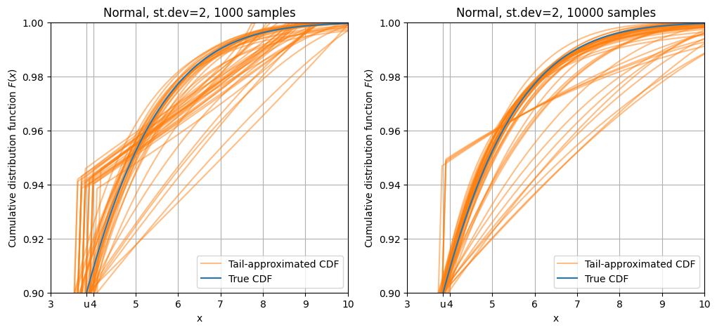
Curves based on 1000 sample points3 (left panel) show a lot of variation. The normal distribution tail falls off rapidly as \(\mathrm{e}^{-x^2}\), so there are very few points on the far tail, which makes the fit very variable. Curves based on samples with size 10000 (right panel) are more aligned with the true CDF.
3 remember that only about 100 of them are above the threshold
Exponential distribution
The exponential distribution’s tail does not fall as quickly as the normal, so most of the approximated curves are around the parent CDF curve.
Show the code
plt.figure(figsize=(12,5))
plt.subplot(1,2,1)
plot_dist(stats.expon(scale = 2), 1000, "Exponential, scale=2, 1000 samples", q=0.9, repeat=50)
plt.subplot(1,2,2)
plot_dist(stats.expon(scale = 2), 10000, "Exponential, scale=2, 10000 samples", q=0.90, repeat=50)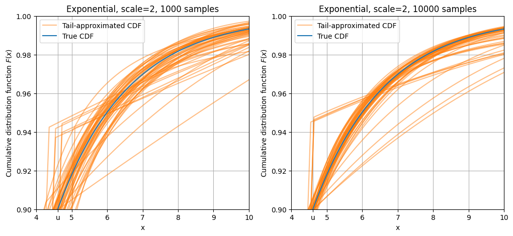
Pareto distribution
Finally, the Pareto distribution has a fat tail, falling off as a negative power: \(F(x; b) = 1 - \frac{1}{x^b}\)
This is also known as a power law.
Because of this fat tail, there are a significant number of points in higher values. As a result, tail approximations have smaller variation.
Show the code
plt.figure(figsize=(12,5))
plt.subplot(1,2,1)
plot_dist(stats.pareto(b = 2.5), 1000, "Pareto, b=2.5, 1000 samples", q=0.9, repeat=50)
plt.subplot(1,2,2)
plot_dist(stats.pareto(b = 2.5), 10000, "Pareto, b=2.5, 10000 samples", q=0.9, repeat=50)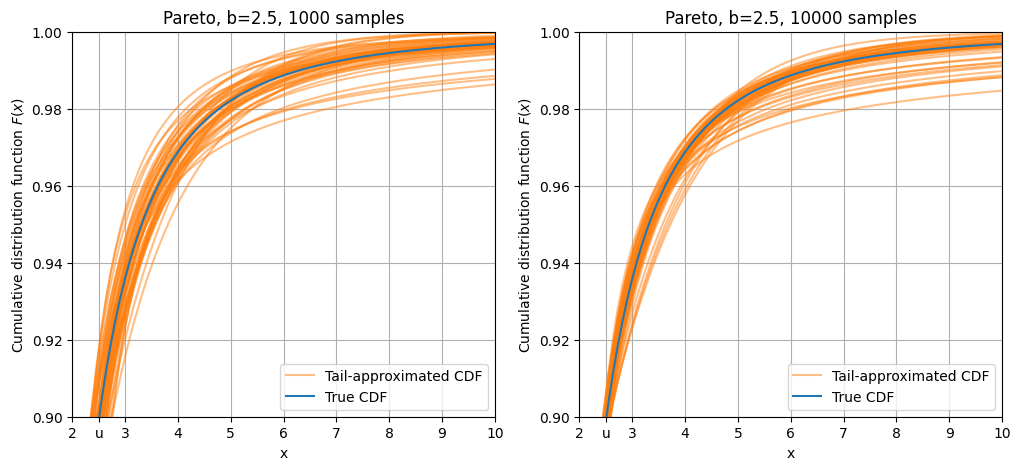
What about multivariate distributions?
The classic discussion above applies to a single random variable. How about the jont extreme-value distribution of several variables, \(F(x_1, x_2,\cdots,x_n)\)?
Multivariate theory of extreme values is more complicated, involving fitting the dependency structure and combining them with copulas. For an example, see Dutfoy et al. (2014)4
4 Dutfoy, Anne, Parey, Sylvie and Roche, Nicolas. “Multivariate Extreme Value Theory - A Tutorial with Applications to Hydrology and Meteorology” Dependence Modeling, vol. 2, no. 1, 2014, pp. 000010247820140003. https://doi.org/10.2478/demo-2014-0003
As a pragmatic alternative, we can first convert the multidimensional data points into scalar anomaly scores. These can be obtained by using anomaly detection methods such as Isolation Forest and Local Outlier Factor, or by evaluating the Mahalanobis distance of data points. Then, we can construct a tail distribution based on these scores. However, this is out of the scope of this post.